Topic covered:

Introduction

Spectral Domains

Convolutional Graph Neural Networks

Spectral CNN

ChebNets or Chebyshev Spectral CNN

CayleyNets

GCN

Special Points on GCN

Some results and analysis

Problems with spectral domains

Conclusions

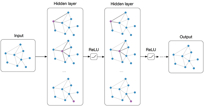
Multi-layer Graph Convolutional Network (GCN) with first-order filters.
Image taken from blog "Graph convolution network by Kipf"

Note

This post includes only basic graph convolution algorithms. It donot include applications of graphs and other algorithms.

Introduction

The great success of Neural Networks for pattern recognition and data mininghas made the researchers to use it in areas like feature engineering, classification etc. Deep architectures like CNN and RNN has revolutionized their use in every domainin which they can be used like text, images, video, signal etc. CNN brought great success on image analysis. The grid structure of image make CNN to exploit local connectivity, translational invariance and shifting to produce meaningful embeddings(low dimensional features) of that image. The growth in computational power and availability of big data are also behind success story of deeplearning architectures.

Researchers thought of using convolution(CNN) on non-grid, irregular structures like graphs. As most ML algorithms needs euclidean distance as similarity notion. Same notion can't be utilised in graphs as it has relative positions. Motivated by CNN, an image can also be thought as special case of graphs where pixel are connected to adjacent pixels.

In graph convolution, one may think as weighted average of node's neighbourhood information. In this post, we will go through graph convolution which has origin in spectral domains.

Spectral Domains

Spectral based methods have solid backing of mathematical foundation in graph signal processing. It assumes that graph is undirected. It uses graph signals and eigen vectors of graph Laplacian matrix. The Global structure can be exploit with spectrum of graph Laplacian to generalize convolution operator.

Mathematically Laplacian has these 3 different forms:

The unnormalized graph Laplacian matrix is defined as
$L = D - A$
The normalized graph Laplacian symmetric matrix is defined as
$L_{s y m} = D^{- 1 / 2} L D^{- 1 / 2} = I - D^{- 1 / 2} A D^{- 1 / 2}$
The normalized graph Laplacian matrix based on random walk is defined as
$L_{r w} = D^{- 1} L = I - D^{- 1} A$

A is Adjacency matrix(may be weighted or unweighed matrix).

A_{i j} = \{\begin{matrix} 1 & edge exists between node i and node j \\ 0 & otherwise \end{matrix}

D is Degree matrix, also diagonal matrix defined

D_{i} = \sum_{j = 0}^{n - 1} A_{i j}

Some properties of L, L_sym and L_rw are :

for every vector $f \in R^{n}$ we have
$f^{T} L f = \frac{1}{2} \sum_{i, j = 1}^{n} A_{i j} {(f_{i} - f_{j})}^{2}$ $f^{T} L_{s y m} f = \frac{1}{2} \sum_{i, j = 1}^{n} A_{i j} {(\frac{f_{i}}{\sqrt{d_{i}}} - \frac{f_{j}}{\sqrt{d_{j}}})}^{2}$
L is symmetric and positive semi definite.
Smallest eigen value of L is 0 and corresponding eigen vector is 1 vector.
Multiplicity k of eigen value 0 of L, L_sym, L_rw is equal to number of connected component in the graph.

Ideal behind using spectral domains is Convolution is easy in signal domain. One application where it is used predominantly is spectral clustering. We will look into it in detail in some other post. One can go through this paper by Luxburg for more details.

Convolutional Graph Neural Networks

As in above paragraph we have different mathematical definitions for graph Laplacian matrix. For simplicity take
$f^{T} L_{} f = \frac{1}{2} \sum_{i, j = 1}^{n} A_{i j} {(\frac{f_{i}}{\sqrt{d_{i}}} - \frac{f_{j}}{\sqrt{d_{j}}})}^{2}$ this is symmetrical Laplacian matrix, also a positive semidefinite matrix.
By diagonalization $L = U Λ U^{T} where U = [u_{1}, u_{2} . . . u_{n}] \in R^{n \times m}$ is matrix of eigen vectors and $Λ$ is a diagonal matrix of corresponding eigen values.

In graph signal processing, a signal is node feature defined as $X_{i} where i \in [n] (n is numbers of nodes)$ .
The Graph fourier transform to a signal X is : $F (x) = U^{T} x$
Inverse graph fourier transform is $F^{-1}\left(\hat{x}\right)= U\hat{x}$ where $\hat{x}$ is resulted signal from graph fourier transform. Here GFT project x into a orthogonal basis formed by eigen vectors of normalized Laplacian. $\hat{x}$ contain element in new feature domains.
So graph convolution is defined as: $F_{G} (x) = x *_{G} g$ where $g$ is convolution filter. $x *_{G} g = F^{- 1} (F (x) ⊙ F (g)) = U (U^{T} x ⊙ U^{T} g)$ All graph spectral convolution follow this same mathematical expression with some approximations.

Spectral CNN

In paper Spectral Network and Deep locally connected network on Graph by Bruna, it is specifically written to use first d eigen vectors of Laplacian matrix which carry smooth geometry of graph. The cutoff frequency d depends on intrinsic regularity and sample size. Here spectral CNN assumes $g_{θ} = θ_{i j}^{k}$ is set of learnable parameters and consider graph signal with multiple channels.
Hence the Graph Convolution layer of Spectral CNN is defined as : $H_{:, j}^{k} = σ (\sum_{i = 1}^{k} U θ_{i j}^{k} U^{T} H_{:, i}^{k - 1}) where (j = 1, 2, . . . f_{k})$ k is the layer index, $H_{:, j}^{k} = σ (\sum_{i = 1}^{k} U θ_{i j}^{k} U^{T} H_{:, i}^{k - 1}) where (j = 1, 2, . . . f_{k})$ is the input graph signal, $H_{0} = X, f_{k - 1}$ is number of input channels, $f_{k}$ is the number of output channels.

It has one big problem, eigen value decomposition is too expensive so it must be replaced by some approximations.

ChebNets or Chebyshev Spectral CNN

Now comes an evolution called ChebNets. It approximate the graph filter $g_{θ}$ by Chebyshev polynomial. $g_{\theta} = \sum_{i=0}^{K}\theta_iT_i(\hat{\Lambda})$ where $\hat{\Lambda} = \frac{2\Lambda}{\lambda_{max}}- I_n$ value of $\hat{\Lambda}$ lie in [-1,1].
The Chebyshev Polynomial is defined by :
$T_i(x) = 2xT_{i-1}(x) - T_{i-2}(x), T_0(x) = 1, T_1(x) = x$
As a result new convolution of signal x is defined over filter $g_{θ}$ is : $x*_Gg_{\theta} = U(\sum_{i=0}^{K}\theta_{i}T(\hat{\Lambda}))U^Tx$

It depends only on nodes that are K-step away from central node (K^th-order neighbourhood). Here getting eigen vector matrix U is still expensive, one solution is to use parametrize $g_{\theta}(\hat{L})$ which recursively use L in place of $\Lambda$ .
As we know $(U Λ U^{T})^{k} = U Λ^{k} U^{T}$
Hence $T(\hat{L}) = U^TT({\hat{\Lambda}})U$ .
Now the Graph Convolution becomes $x*_Gg_{\theta} = \sum_{i=0}^{K}\theta_{i}T_i(\hat{L})x$ where $\hat{L} = \frac{2L}{\lambda_{max}}-I_n$ .
The Spectrum of Chebnet is mapped to [-1, 1] linearly. It is great improvement over spectral CNN. Also K^th of Laplacian is exactly K-Localized. Above derivation of expression is too much concentrating as i thought it would be better to show how we remove U which is necessary as it is too expensive to compute.

CayleyNets

CayleyNets is another convolution framework over graph. CayleyNets futher applies Cayley polynomials in place of Chebyshev Polynomial. Cayley polynomials are parametric rationan complex to capture narrow frequency bands.
The spectral convolution of CayleyNets is defined as: $x *_{G} g_{θ} = c_{0} x + 2 R_{e} \{\sum_{j = 1}^{r} c_{j} (h L - i I)^{j} (h L + i I)^{- j} x\}$ $R_e(.)$ is real part of complex numbers.
$c_0$ is real coefficient.
$c_j$ is complex coeffiecient.
$h$ control the spectrum of Cayley filter.

Graph Convolutional Network

Now we come to most simpler part of convolution on graph which is easy to understand and apply. Although CayleyNets works well nut its too complex equation to understand. It introduces first order approximation of ChebNets.
As we know in last post that Chebnets equation is given by : $x*_Gg_{\theta} = \sum_{i=0}^{K}\theta_{i}T_i(\hat{L})x$
Setting K = 1, we have $x*_Gg_{\theta} = \sum_{i=0}^{1}\theta_{i}T_i(\hat{L})x$
From Chebyshev polynomial defined in ChebNets section we know that $T_0{x} =1, T_1(x) =x$

Expanding above equation we get :

$x*_Gg_{\theta} = \sum_{i=0}^{1}\theta_iT(\hat{L})x \Rightarrow\theta_0T_0(\hat{L})x+\theta_1T_1(\hat{L})x$
$\Rightarrow\theta_0T_0(\hat{L})x+\theta_1T_1(\hat{L})x$
$=\theta_0x+\theta_1(\hat{L})x$
$\Rightarrow \theta_0x+\theta_1(I_n-D^{-\frac{1}{2}}AD^{-\frac{1}{2}})x$
$\Rightarrow (\theta_0+\theta_1)x - \theta_1D^{-\frac{1}{2}}AD^{-\frac{1}{2}}x$

An assumption $\theta = \theta_0 = -\theta_1$ , has been taken to reduce the parameters from overfitting
So overall equation for Graph Convolution reduced to : $\Rightarrow D^{-\frac{1}{2}}AD^{-\frac{1}{2}}x$

One more thing left is self loop, so when we include self loop new Adjacency matrix is : $\hat A = A+I_n$
Now $D^{-\frac{1}{2}}\hat AD^{-\frac{1}{2}}$ has eigen values in [0, 2], repeated operation of this can lead to numerical instabilities along with exploding and vanishing gradient when used in Deep Neural Network models.

To alleviate this problem, Renormalisation trick is used. In Renormalisation trick, we replace $D$ with $\hat D$ where $\hat D$ is defined as: $\hat D_i = \sum_{j =0}^{n-1}\hat A_{ij}$ and $\hat A$ is new Adjacency matrix.

Now the main graph convolution expression with all improvement is:
$Z = \hat D^{-\frac{1}{2}}\hat A \hat D^{-\frac{1}{2}}X\theta$
$Z \in R^{N\times F}$ is convolved signal matrix.
$\hat Ax$ can be efficiently implemented as product of sparse matrix with dense matrix.

The whole derivation might be confusing for first time. If going by simple intution we know that a a classifier (may be shallow neural network or Logistic classifier) can be $f(\theta x)$ where f is some non linear function like sigmoid/Relu/Softmax etc, $\theta$ is learnable parameters(weights) and $x$ is the feature vector.

In GCN we simply replace $x$ with $\hat Ax$ . By doing this we are aggregating all the features of nodes in neighbourhood. Some nodes has small number of neighbours while some has large neighbourhood, so aggregated features may not scale properly, hence we used normalised Laplacian to make them in same range.

$f(\theta \hat D^{-\frac{1}{2}}_{i}\hat A_{ij}\hat D^{-\frac{1}{2}_{i}}X)\Rightarrow f(\theta \frac{1}{n_i}\sum_{j \in N(i)\cup i}x_j)$ this equation is showing us that we are simply taking aggregate mean of node features along with neighbour's node features. This equation is first order approximation of ChebNet with some improvement. It is the expression for single layer of Graph Convolution Networks. To get K^th order Graph Convolution filter we can stack K layers of GCN. K layer of GCN stacking is simply like K layer MLP.

In the original paper of GCN by Thomas Kipf, ReLu is used as Non-linear activation function. In paper SGC(Simplifying-GCN , it is written that non-linear function contribution to actual performance is very less, main contribution comes from local averaging of node features. By doing this way they have shown to reduce the complexity too much resulting in too less training time(as linear classifier trained easily in less time ) and above or at par performance than original GCN.

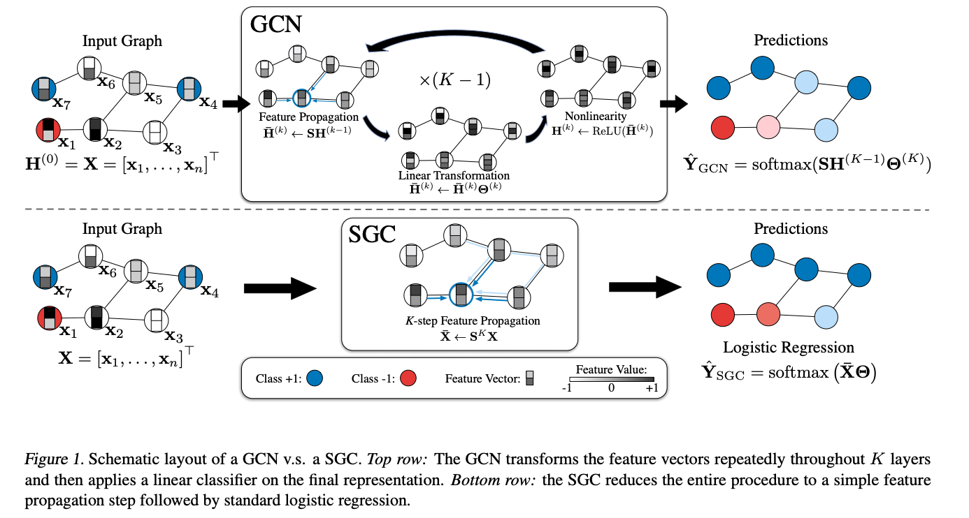
this figure is taken from SGC paper , It tells us about the how SGC and GCN works

There are some other modificatios of GCN like Large-Scale Learnable Graph Convolutional Networks, Attention-based graph convolutional networks, Dynamic Graph Convolutional Network etc. which we will not discuss here.

Some results and analysis

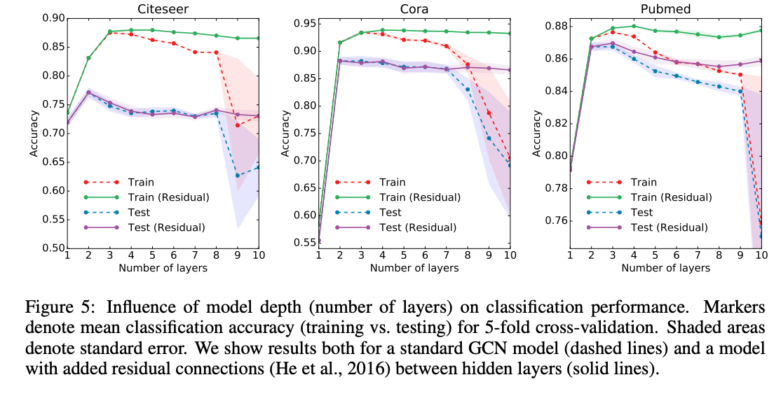
This image is taken from GCN paper(mentioned in reference).
It show how the performance vary with respect to number of layers on 3 data sets Cora, Citeseer, and Pubmed.

We can see from the figure that stacking large numbers of GCN layer make the model overfit on all dataset, this is due to high complexity. The best result is when two layers are stacked togethers. For GCN layer stacked greater than 2, perfomance either remain constant or got overfit. For count of GCN layers less than 2, model got underfit.

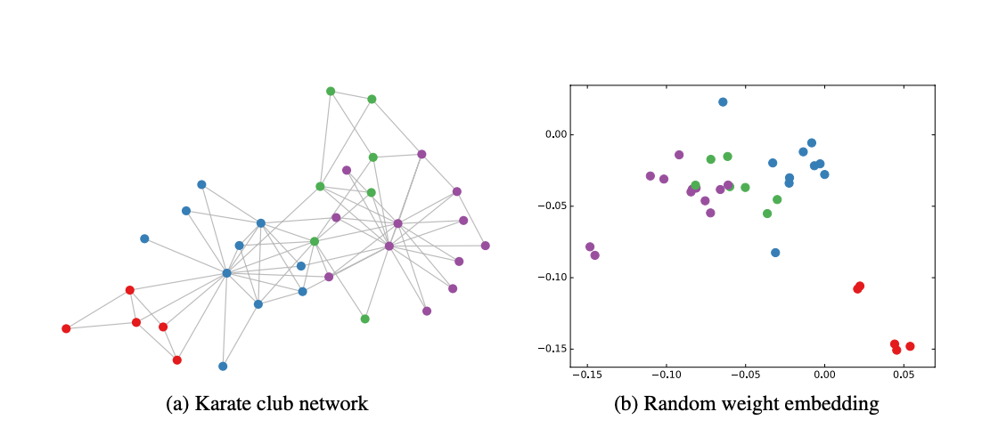
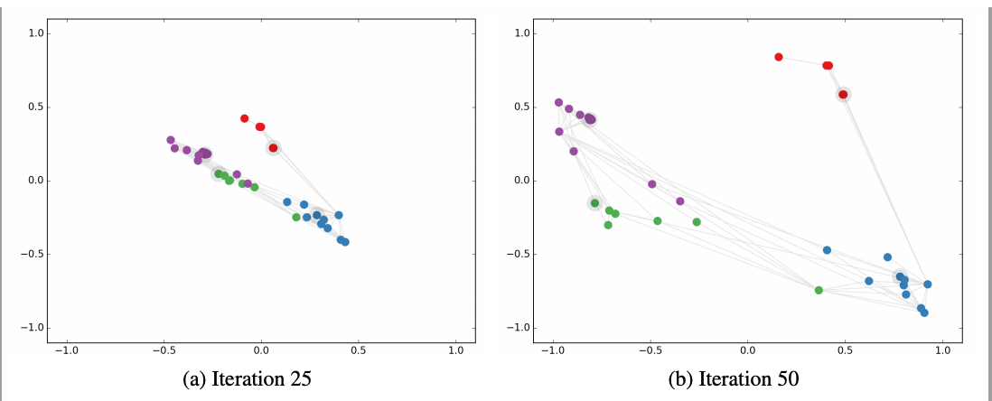
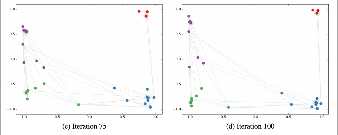
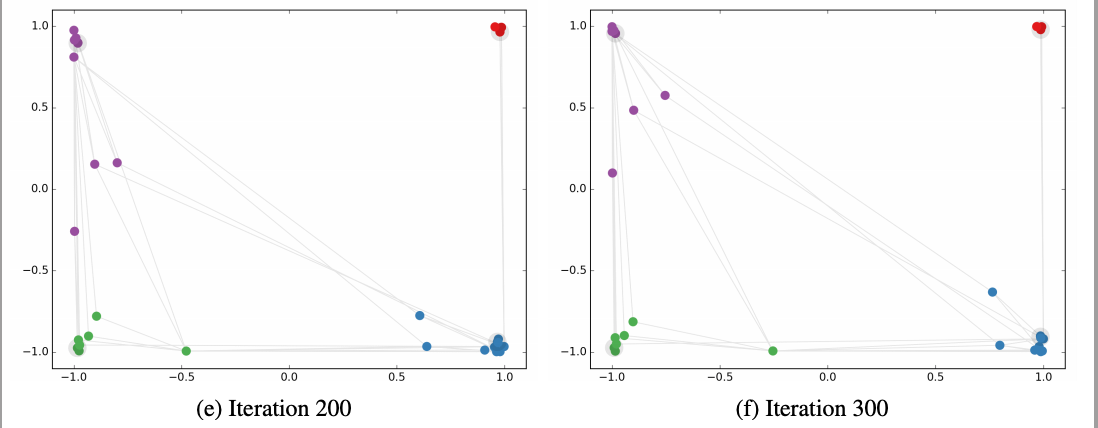
This image taken from GCN paper. It show how embedding on dataset mentioned Karate Club
projections change as GCN get trained with respect to iterations

Above image shows the embedding projections of nodes in Karate club graph. As GCN got trained, the similar nodes are getting more closer. Movement of forming clusters can be notice with respect to iterations.

Performance of different Frameworks using Graph Convolution in spectral domain on the 3 dataset mention in table below

Framework	Accuracy on Cora Dataset	Accuracy on Citeseer Dataset	Accuracy on Pubmed Dataset
ChebNets	81.2%	69.8%	74.4%
GCN	81.5%	70.3%	79%
CayleyNets	81.9%	-	-
SGC	81%	71.9	78.9%

The result mention taken from standard papers result portions like GCN, SGC, GAT etc. From result we can see that GCN improvement make the perfomance increased by some points with respect to ChebNets. CayleyNets is better than GCN on Cora. Lastly SGC mentioned above is at par with respect to GCN with too much reduced complexity and faster training.

Special points about GCN

From results and analysis section, good results is found by stacking 2 layers, more than that cause either no change or overfitting.
In random graphs, one can have maximum of diameter of 6 which restrict us not to use more layer of GCN as it will make all nodes feature alike.

Problems with spectral domains

Highly complex and inefficient, although GCN is effiecient.
Spectral models rely on graph fourier basis which generalises poorly on new graphs. They assume fixed graph, any peturbation would change the eigen basis.
Spectral models are only used for undirected graphs, so flexibilty remains less as can't be used for other types of graphs.

Conclusions

I tried to be flexible, only covering graph convolution related with spectral domains. Some part of the post are more theoritical which are not understandable in one go, for that i have mark some paper in references. I don't go through other parts like training. All models are trained in similar fashion like simple neural network with backpropagation and cross entropy as loss functions. In some other post, i will go through in details about practical applications of graph.

There are other algorithms in graph machine learning not originated in spectral domains like random walks based method e.g. Deepwalk, Node2vec, SDNE, LINE etc.

Reference

From

Swyam Prakash Singh, ML enthusiast

Evolution of Convolution on Graphs(spectral Domains)

Topic covered:

Note

Introduction

Spectral Domains

Some properties of L, Lsym and Lrw are :

Convolutional Graph Neural Networks

Spectral CNN

ChebNets or Chebyshev Spectral CNN

CayleyNets

Graph Convolutional Network

Some results and analysis

Special points about GCN

Problems with spectral domains

Conclusions

Reference

From

Some properties of L, L_sym and L_rw are :